LIVE · BITSTAMP BTC/USD

The Bitcoin halving cycle, measured.

Bitcoin runs on a ≈4-year clock. Bottoms have struck ≈524 days before each halving, tops ≈535 days after. This site measures that clock on real data — and shows you, in one live chart, two simple scores and a daily report, exactly where today sits.

Phase now 1 of 10 cycle phases
Opportunity 0–100 · higher = better odds
Heat 0–100 · higher = more risk
Next daily report posted 08:10 Berlin, every day

No account. No install. Your settings stay in your browser.

BOTTOM −524d ±16 TOP +535d ±11 BOTTOM→TOP 1,059d ±9 BEAR 383d ±21 DECAY ×0.27 / CYCLE POWER LAW R² 0.96 HALVING ≈ MIDPOINT ×1.02 TOPS 81–83% OF FIT CEILING ABSORPTION ×2.5 ISSUANCE NUPL TOPS ≥0.65 · BOTTOMS ≤−0.28 BOTTOMS BELOW THE LTH FLOOR BOTTOMS: ≥98.6% STH IN LOSS 10 PHASES · 4 ENGINES 3 SYSTEMS · 1 CONSENSUS 67.4% DIRECTIONAL · N=371 OUT-OF-SAMPLE 4 HALVINGS · 15 YEARS OF DATA
01 · THE CYCLE

One rhythm, four times in a row

Bitcoin's supply halves roughly every four years. Around each halving, price has traced the same anatomy — measured here on real data, not folklore.

BOTTOM −524d ±16 HALVING the midpoint · ×1.02 ±0.05 TOP +535d ±11 1,059 days bottom → top · varies by just ±9 days across the last three cycles
Measured on Bitstamp + Coin Metrics history, cycles 2016 / 2020 / 2024. The ±500-day calendar rule brackets exactly this structure.
0days, bottom → top
(CV 0.8%)
0days before halving
the bottoms struck
0days after halving
the tops printed
0days of bear market,
top → next bottom
0the multiple each cycle
keeps of the last (R² 0.998)
02 · THE INSTRUMENT

Everything on the chart is a switch

Start with a clean TradingView-style chart. Layer on exactly the evidence you want — every toggle remembers your choice, privately, in your own browser.

AThe 500-day rule, drawn live

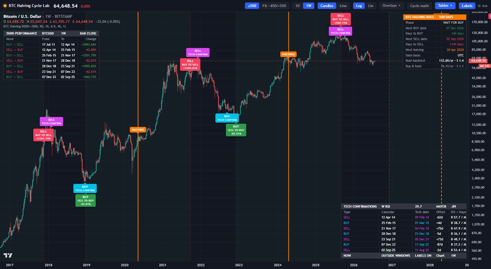
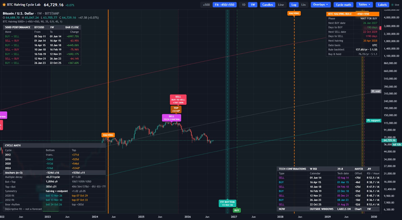
Halving lines, BUY/SELL dates with every historical move measured close-to-close, technical confirmations, and the research tables — over live candles that tick with every Bitstamp trade. Layer any of 18 evidence overlays, sketch your own ideas with the built-in drawing tools, and read it on four timeframes. The current bar forms in front of you, with a countdown to the close.

  • 4 timeframes
  • 18 overlays
  • Drawing tools
  • Candles / Line
  • Log / Linear
  • Labels & tables on/off
The live halving-cycle chart with BUY/SELL labels, halving lines, and research tables

BCycle math, on demand

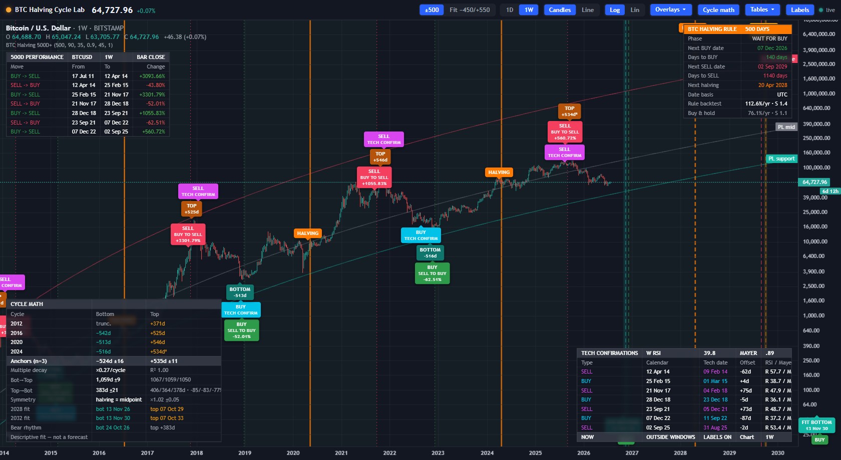
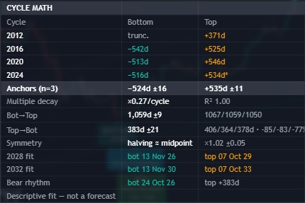
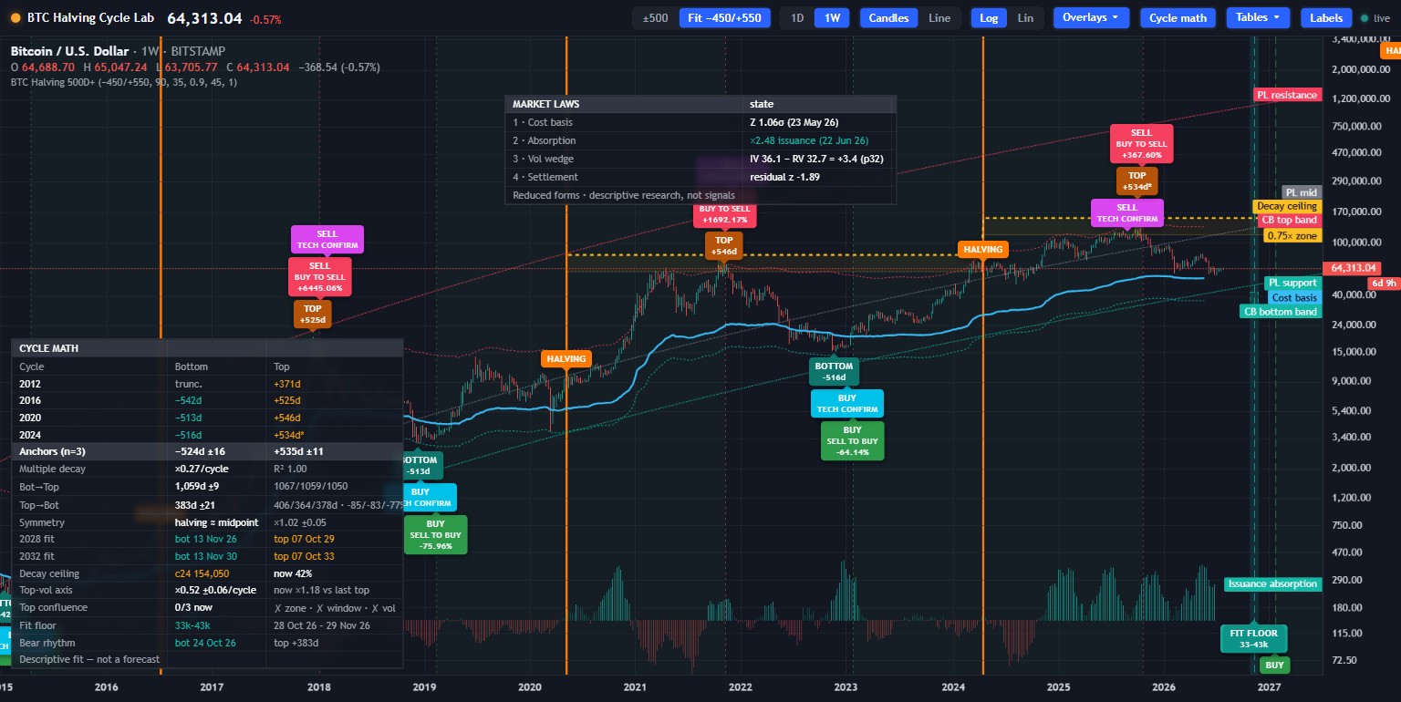
One click marks every measured bottom and top with its distance from the halving, shades the fitted windows for the 2028 cycle, and opens the CYCLE MATH panel — anchors, decay law, rhythm constants. The Decay Ceiling draws each cycle's causally-projected top zone (both testable tops printed at 81–83% of it), and a fitted floor box brackets the forming bear bottom. All labeled for what they are: hindsight fits, not forecasts.

  • Cycle math
  • Decay ceiling
  • Power-law corridor
  • 200W / 200D SMA
  • Pi Cycle
Cycle math overlay: measured bottoms and tops, fitted 2028 zones, power-law corridor

CTwo rules, one click

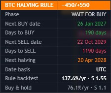
The classic ±500-day rule ships untouched. Next to it: a research preset fitted to the measured anchors — buy 450 days before, sell 550 after — with its full backtest shown right on the chart, honestly compared against buy & hold.

Rule table with backtest: 137.6%/yr, Sharpe 1.55 vs buy and hold 76.1%/yr Cycle math panel with anchors, decay and projections
Fitted rule view with projected windows and backtest

DFive market laws, honestly graded

Reduced-form implementations of five candidate mathematical laws of Bitcoin — cost-basis elasticity (network cost basis with dispersion-normalized bands: tops are measurably more stable in Z than in raw MVRV), halving absorption (net coins leaving exchanges per unit of new issuance — flips positive after every modern halving; ×2.5 right now), a volatility wedge, a security-settlement manifold, and a dormancy-release hazard — graded on the full on-chain history: NUPL separated every measured top (≥0.65) from every measured bottom (≤−0.28), n = 3+3. The MARKET LAWS panel shows each law's live state and its verdict — including the ones our data can't confirm. A research tool that grades its own homework.

  • Cost basis bands
  • Issuance absorption
  • Regime ribbon
  • Market laws panel
  • Deribit DVOL
  • ✓✓ confirmed · ✗✗ not
Market laws panel with cost basis bands, issuance absorption histogram, and verdicts
03 · THE COMPASS

Where are we right now? Two numbers.

The Cycle Regime Map splits the 4-year cycle into ten named phases and checks the calendar's claim against four independent confirmation engines. Everything rolls up into two scores anyone can read — live, below.

  1. Cycle exhaustion
  2. Deep accumulation
  3. Recovery expansion
  4. Mid-cycle reset
  5. Pre-halving markup
  6. Post-halving digestion
  7. Main bull expansion
  8. Euphoria & distribution
  9. Bear-market transition
  10. Capitulation & bottom search

Ten phases, anchored to the halving clock. The lit pill is today.

OPPORTUNITY

fetching the live score…

How attractive current conditions score against the measured past, 0–100. A weighted read of timing, valuation, technicals, holder behavior, liquidity and leverage — each weight published.

HEAT

fetching the live score…

How overheated the market looks, 0–100. High heat is a risk reading, never an entry signal — the site tells you that on every surface where the number appears.

Live snapshot · confidence /100 · every component and weight is on the dashboard

Technical —/100

Price trend and momentum: Mayer Multiple, weekly RSI, MACD, drawdown, volatility.

On-chain —/100

What holders are actually doing: MVRV, NUPL, reserve risk, cost-basis floors, miners.

Liquidity —/100

Money flowing in or out: exchange flows, issuance absorption, ETF demand, macro.

Derivatives —/100

Leverage and froth: funding rates, open interest, implied volatility.

04 · THE SECOND OPINION

Three systems. One honest answer.

The calendar is only one opinion. Two more systems read the market with no calendar at all — and the site shows you where all three agree, and where they don't.

The calendar

Counts days around the halving. Simple, transparent, testable — the ten-phase clock you saw above.

Phase table + the ±500-day rule, versioned and backtested.

The statistician

Names the market's state purely from the data's behavior — and flags the exact moment that behavior shifts.

Hidden Markov regime probabilities + Bayesian change-point detection, no lookahead.

The historian

Hunts the past for stretches that look most like today — then shows what happened next, with sample sizes.

Multivariate DTW historical analogues + phase similarity.

When they disagree, we show you

Calendar
Statistician
Historian
  • calendar × statistician:
  • calendar × historian:
  • statistician × historian:

The live three-way read loads a moment after the page. Divergence is a finding, not an error: it means a transition may be under way — or this cycle is behaving unlike the measured past.

combined confidence /100 · never averaged away, always shown

05 · THE FORECAST LAB

Forecasts that had to earn it

Every model here is tested the hard way before you ever see it: trained only on the past, graded only on data it never saw. Its report card is public.

0%

directional accuracy — walk-forward, out of sample

371 ninety-day forecasts · 24 folds across 15 years · beats every naive baseline it was tested against

Ranges, not price targets

p90 p50 p10

A forecast here is a distribution — quantiles with probabilities, resampled from every comparable moment in history. Never a single magic number. Under 30 samples, the page says so and widens honestly.

Drawdown odds, stated first

Before anything else, the lab states the measured chance of a painful drop inside the forecast window — not just where price might end.

  • P(−10%)
  • P(−20%)
  • P(−30%)
  • worst excursion, not endpoint

Model health, public

Data freshness, drift, out-of-distribution and structural-break monitors — one Model Health dashboard, refreshed daily. When inputs degrade, confidence drops and the page tells you why.

Shadow mode

New models predict in public but cannot touch the production scores until their out-of-sample record earns promotion. Predictions are stored before their outcomes exist — no backtest subtlety can contaminate them.

06 · THE METHOD

How it calculates

The whole pipeline is deterministic and inspectable — the same numbers every time, from public data you can check yourself.

  1. 1

    Public data, kept fresh

    Full Bitstamp BTC/USD daily history, extended back to 2010 with Coin Metrics community data. The chart re-syncs itself minutes after every UTC bar close.

  2. 2

    The calendar rule

    BUY = halving − offset · SELL = halving + offset. Every completed BUY→SELL and SELL→BUY move is measured close-to-close and listed in the performance table — including the drawdowns.

  3. 3

    Technical confirmations

    Only completed weekly bars count — no repainting. BUY: weekly RSI(14) crosses above 35 while the Mayer Multiple ≤ 0.90. SELL: weekly MACD turns bearish while RSI ≥ 45 and Mayer ≥ 1.00, within ±90 days of a calendar date.

  4. 4

    Cycle research fits

    Bottoms and tops located per cycle → anchor statistics, the ×0.27 decay law, a log-log power-law corridor (R² 0.96), and projected 2028 windows — every fit shown with its sample size and dispersion.

  5. 5

    Walk-forward validation

    Models train only on the past and are graded on data they never saw — 371 out-of-sample 90-day forecasts behind the accuracy number above. New models wait in shadow mode until their record earns promotion.

07 · THE DAILY RHYTHM

It reports in, every single morning

No refresh-watching required. The lab publishes its read once a day — short, visual, and free — and the full report is one click away at any hour.

The daily post on X

Every morning at 08:10 Berlin time, the bottom checklist and both scores go out as one clean card on X — the same numbers this page reads, drawn by the same code.

next post in

Follow @Derik_vt on X

The analysis report

The bottom checklist and the model intelligence read, generated fresh from live data the moment you click — a clean PDF you can file, print or forward.

Generate analysis report (PDF)
08 · THE TOOLKIT

Every tool, explained — simply and precisely

Each layer on the chart in one plain sentence, with the exact math and its intended use one click away. Nothing is a black box, and nothing here is financial advice. See them all combined on the Cycle Dashboard.

The ±500-day rule rule · “±500”

Buy 500 days before each halving, sell 500 days after. That is the entire rule — and it beat holding in every completed cycle.

The math & how to use it

BUY = halving − 500d · SELL = halving + 500d. Moves are measured close-to-close; the backtest is long BTC inside the windows, cash outside, 0.1% cost per switch: 112.6%/yr, Sharpe 1.40 vs buy-and-hold 76.1%/yr, Sharpe 1.10.

Use: the baseline. Everything else on the chart exists to confirm or challenge these two dates.

The fitted −450/+550 rule rule · “Fit”

The same idea, tuned by a backtest scan around the measured anchors: buy a little later (after the average bottom has already printed), sell a little later.

The math & how to use it

Offsets from an offset-sensitivity scan over the measured anchors: BUY = halving − 450d · SELL = halving + 550d137.6%/yr, Sharpe 1.55, max drawdown −74.8%. An in-sample fit on three cycles — versioned, never silently replacing the classic rule.

Use: a research preset to compare against ±500, with its backtest shown on the chart.

Technical confirmations labels · on by default

The calendar says “around here”; momentum says “now”. The aqua and fuchsia flags mark when weekly momentum agreed with a BUY or SELL date.

The math & how to use it

Completed Sunday-close weekly bars only — no repainting. BUY: weekly RSI(14) crosses above 35 while the Mayer Multiple (price ÷ 200-day SMA) ≤ 0.90. SELL: weekly MACD(12,26,9) crosses bearish while RSI ≥ 45 and Mayer ≥ 1.00 — each within ±90 days of a calendar date; only the first hit per window is kept.

Use: timing refinement inside the calendar windows.

Cycle math — anchors & rhythm toggle · Cycle math

In the last three cycles the bottom struck ~524 days before the halving and the top ~535 days after — and bottom-to-top took almost exactly 1,059 days every time.

The math & how to use it

Extremes located per cycle, then averaged: bottoms −524d ±16, tops +535d ±11, bottom→top 1,059d ±9 (0.8% variation), bears 383d ±21 at −77…−85%, and the halving sits at the temporal midpoint (ratio 1.02 ±0.05). Future zones are drawn at mean ±1σ.

Use: the “when” scaffolding — fitted bottom Oct–Nov 2026, fitted top around Oct 2029.

Decay ceiling toggle · Decay ceiling

Each cycle’s pump is a shrinking fraction of the previous one. Projecting that shrinkage gives this cycle a price ceiling — known on halving day, before it happens.

The math & how to use it

Ceiling = halving-day price × decay-projected multiple, where the multiple is a log-linear extrapolation of prior completed cycles’ halving→top multiples (×92.6 → ×29.6 → ×7.9, decaying ×0.27 per cycle). Causally testable twice: the 2021 top hit 83.2% of its ceiling, the 2025 top 81.0%. The dotted line marks the 0.75× terminal zone; amber boxes show where the zone crosses the calendar top window — both real tops died inside their box.

Use: a level zone, not a timing signal — it means most inside the calendar top window.

Fit floor with Decay ceiling

The same shrinking-cycle logic pointed downward: a falsifiable target box for where this bear could bottom.

The math & how to use it

Two independent estimators bracket the zone: the bear-depth trend (−84.9% → −83.4% → −76.7% → next ≈ −73.5% of the top) and the bottom ÷ previous-halving-price ratio decay (14.0 → 4.9 → 1.8 → next ≈ 0.66×) → $33k–43k, drawn across the fitted Oct–Nov 2026 window. Never tested out of sample.

Use: a concrete box to be proven right or wrong — note this bear is already shallower than every precedent, so a shallow miss is the live risk.

Power-law corridor toggle · Power-law corridor

Across its whole life, Bitcoin’s price has grown along a straight line — once you plot both price and age on logarithmic scales. The corridor brackets that line.

The math & how to use it

log₁₀(price) = a + k·log₁₀(days since genesis) with k = 5.66, R² = 0.96; support, mid, and resistance sit at the 1st/50th/99th percentiles of the fit residuals.

Use: long-horizon context — every bear-market bottom (2015, 2018, 2022) held inside the corridor, 36–81% above the support line.

Cost basis bands — Law 1 toggle · Cost basis bands

The blue line is what the average coin last changed hands for — the market’s collective cost basis. Price stretches away from it and snaps back.

The math & how to use it

Realized price = price ÷ MVRV. The deviation is normalized by its own 4-year dispersion: Z = ln(MVRV) ÷ σ₄ᵧ. Measured result: tops cluster at Z ≈ 2.74 with far less spread than raw MVRV (CV 0.19 vs 0.33), while bottoms are tightest in raw MVRV (≈0.68). Bands: cost basis × e2.74σ (top) and × 0.68 (bottom).

Use: how hot or cold price is versus what holders actually paid — the bottom band independently agrees with the fit floor.

Issuance absorption — Law 2 toggle · Issuance absorption

Are buyers soaking up more coins than miners create? Above 1 on the histogram means yes — a supply squeeze.

The math & how to use it

(exchange outflows − inflows, 90d avg) ÷ (new issuance in USD, 90d avg). It flipped positive in the year after every modern halving (−0.21→+0.09, −0.75→+0.19, −0.34→+0.20) and currently reads ×2.48 — historically extreme accumulation.

Use: a flows-based leading gauge; strong absorption during weak price is the classic accumulation signature.

Volatility wedge — Law 3 MARKET LAWS panel

Options traders pay a premium over recent realized chaos; the size of that premium says how nervous the market is.

The math & how to use it

wedge = DVOL (Deribit 30d implied vol) − trailing 30d realized vol, deflated by annualized |funding|. Currently ≈ +3 points (32nd percentile — sleepy). The full invariant needs order-book depth and open interest we don’t have, so its stationarity claim is graded not confirmed — and the panel says so.

Use: context only. A lab that grades its own homework keeps its confirmations credible.

Settlement manifold — Law 4 MARKET LAWS panel

Compares what Bitcoin spends on security (mining) with how much value it settles. Big imbalances should flag stress.

The math & how to use it

ln(issuance ÷ realized cap) ~ ln(settlement value ÷ realized cap); the regression residual is the state. On our community-data proxies the relation is weak (R² 0.08, ~3.5-year half-life) — graded weak, displayed for honesty.

Use: watch, don’t lean on it — it needs adjusted transfer-value data to matter.

Regime ribbon toggle · Regime ribbon

One colored strip that reads all of the above and names the season: accumulation, expansion, distribution, or de-risk.

The math & how to use it

Four agreement-gated blocks: cost-basis Z position between the measured bottom/top thresholds, the cycle leg from the anchors, volatility stress versus expanding percentiles, and absorption > 1. Components that disagree are shown as a “mixed” flag instead of hidden. Example: the Oct 2025 read flipped to DE-RISK — mixed, since absorption still said accumulate; the chart and dashboard always show the live read.

Use: the one-line answer to “where are we?” — the dashboard breaks it into components.

ERCO — elastic repricing oscillator toggle · ERCO

A 0–100 pressure gauge asking three questions at once: how stretched is price above its structural anchor, is that anchor still repricing upward to catch up, and how much of the cycle’s volatility budget is already spent? Stretch is only fragile when the anchor stalls and the budget is gone.

The math & how to use it

X = 1.2·z(ln P/A) − 0.9·z(Δ₉₀ ln A) + 0.8·(2V−1) + 0.35·z(volume impulse), ERCO = 50 + 50·tanh(X/2), smoothed by a 7-day EMA. The anchor A is realized price when on-chain data is fresh, else a price-only hybrid √(200W×730D SMA). V is cumulative squared daily returns since the halving divided by a causal budget — the median spent at prior cycles’ tops only. Measured with the report’s default weights (nothing fitted here): all three measured tops read 71–73 on the realized-price anchor (n = 3), while bottoms drifted 10 → 20 → 35 as the market matured. If the on-chain feed ever goes stale the overlay automatically falls back to a price-only hybrid anchor (tops ≈77/62, n = 2) — and the chart panel always names the active mode. Honestly graded: the report’s prototype trading rules underperform buy-and-hold (realized-price anchor: Sharpe 0.65 vs 1.22; hybrid: 0.60 vs 1.09) — so the lab displays ERCO as a state gauge, never a trade trigger.

Use: read it against the calendar windows — a high read inside a SELL window is top-side confluence; a low read inside the BUY window is accumulation-consistent. The anchor-band overlay draws A·eμ±σ on the price chart.

Dormancy & NUPL toggle · NUPL

Are long-term holders sitting still or starting to spend old coins — and how much paper profit is the market sitting on? In the on-chain literature, tops have come when old coins move while everyone is deep in profit — a pattern our short data window can’t yet verify.

The math & how to use it

NUPL = (market cap − realized cap) ÷ market cap — below 0 is capitulation, above 0.75 is euphoria. Liveliness = lifetime coin-days destroyed ÷ coin-days created; a rising 90-day change means dormant supply is waking up, and a coin-days-destroyed z-score adds spend intensity. The grade is computed from the data window: with at least two completed tops and bottoms in view, the panel reports whether NUPL actually separates them; with a shorter window it honestly says “context only”. The MARKET LAWS panel always shows the current grade.

Use: a top-side sanity check. Distribution warnings need BOTH high NUPL and rising liveliness; neither alone is enough.

Cost-basis ladder toggle · Cost-basis ladder

Two more cost-basis lines with different owners: what short-term holders paid (bull support, bear resistance) and what long-term holders paid — the conviction floor. Where price sits on the ladder tells you who is underwater.

The math & how to use it

STH/LTH realized prices are the average acquisition cost of coins younger/older than ~155 days. Measured on our extremes: every measured bottom printed below the LTH floor — at 0.571×, 0.723× and 0.771× (n = 3, and the ratio rises as the market matures). Alongside Reserve Risk, whose measured bottoms cluster tightly at 0.0004–0.0007 (n = 3; its tops decay, so it grades bottoms only).

Use: structure at a glance — price under the STH line is bear structure; a dip toward or under the LTH floor has marked every generational low.

Modern context: ETF flows & global M2 toggles · ETF / M2

Two forces the old cycles never had: US spot ETFs absorbing (or dumping) coins, and the global money supply everyone claims Bitcoin follows. One is brand new; the other we actually measured.

The math & how to use it

ETF net flows (BTC/week) start Jan 2024 — no historical baseline exists, so they are context, never part of a graded law. The M2 thesis we graded properly: weekly year-over-year changes of BTC vs global M2 show only a weak full-sample correlation with no lead-lag advantage at any horizon up to 40 weeks — the popular “M2 leads by 10 weeks” claim does not hold on this data, though the recent era correlates moderately. The dashboard shows the exact numbers.

Use: ETF flows show whether the new demand channel is buying or selling this month; M2 is macro mood — useful context, honestly graded as nothing more.

Bottom Radar toggles · Floor stack / % STH in loss

Three distinct floor estimators plus the pain gauge, all graded on the measured bottoms. When these methods and the calendar converge on one zone, that’s the strongest read this site can give — and it says so with sample sizes attached.

The math & how to use it

CVDD, Balanced Price and True Market Mean are graded by their measured bottom-ratio bands (price ÷ estimator at the n = 3 bottoms): bottoms never touched CVDD (printed at 2.5–3.4× it), held above Balanced Price at the 2018 and 2022 bottoms (1.23–1.40×) — the 2015 bottom printed 13% below it (0.87×) — and printed at 0.36–0.53× TMM. Implied zone = today’s value × that band. All three derive from the same realized-value / coin-days-destroyed data, so their zones are correlated — methodologically distinct, not independent votes; the calendar is the only independent axis here. The pain gauge: every measured bottom printed with ≥98.6% of short-term holders in loss (n = 3) versus ≤0.5% at tops — the cleanest separation of any gauge on this site. Hash ribbons (miner capitulation) overlapped every bottom ±90d but also fire elsewhere — context only. The dashboard shows the live zones and today’s reads.

Use: watch the dashboard as the consensus bottom window (union of the independent time methods, Oct 2026 – Jan 2027) approaches — the radar shows which conditions are met, never a buy signal.

09 · THE RULES WE FOLLOW

Honesty is the product

Most market sites sell certainty. This one sells measurement — and four rules make that difference real on every page.

RULE 1

Measured, not predicted

Every line is computed from public data with its formula shown. Hindsight fits are labeled as hindsight fits — never dressed up as foresight.

RULE 2

Every number carries its sample size

Three completed cycles is a sample of three. Each claim ships with its n and its spread, right where the number is.

RULE 3

It can say “no reliable signal”

When evidence is thin or systems disagree, the platform says exactly that. A tool that can't say “I don't know” is a marketing site.

RULE 4

Never financial advice

Research and education, nothing else. No calls, no targets, no “buy now”. What you do with the evidence is entirely yours.

Bitcoin has completed three full halving cycles with reliable data. Three of anything is a pattern, not a proof. That is why this chart shows you dispersion, sample sizes, and backtests instead of predictions — and why the current cycle already bends some of the old rules. Research evidence, honestly presented. Never financial advice.

The next fitted window is already on the chart.

Fitted bottom zone: Oct–Nov 2026 · Fitted top zone: Oct 2029 — and the Opportunity and Heat scores are reading today's tape right now.

Open the live chart — free